Introductory Notebook to mpnum

mpnum implements matrix product arrays (MPA), which are efficient parameterizations of certain multi-partite arrays. Special cases of the MPA structure, which are omnipresent in many-body quantum physics, are matrix product states (MPS) and matrix product operators (MPO) with one and two array indices per site, respectively. In the applied math community, matrix product states are also known as tensor trains (TT).

The main class implementing an MPA with arbitrary number of array indices (or “physical legs”) is mpnum.MPArray.

import numpy as np
import numpy.linalg as la

import mpnum as mp

MPA and MPS basics

A convenient example to deal with is a random MPA. First, we create a fixed seed, then a random MPA:

rng = np.random.RandomState(seed=42)
mpa = mp.random_mpa(sites=4, ldim=2, rank=3, randstate=rng, normalized=True)

The MPA is an instance of the MPArray class:

mpa

<mpnum.mparray.MPArray at 0x7f65672eaa90>

Number of sites:

len(mpa)

4

Number of physical legs at each site (=number of array indices at each site):

mpa.ndims

(1, 1, 1, 1)

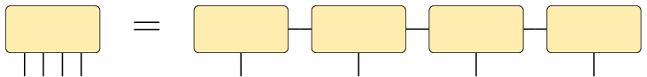
Because the MPA has one physical leg per site, we have created a matrix product state (i.e. a tensor train). In the graphical notation, this MPS looks like this

Note that mpnum internally stores the local tensors of the matrix product representation on the right hand side. We see below how to obtain the “dense” tensor from an MPArray. Dimension of each physical leg:

mpa.shape

((2,), (2,), (2,), (2,))

Note that the number and dimension of the physical legs at each site can differ (altough this is rarely used in practice).

Representation ranks (aka compression ranks) between each pair of sites:

mpa.ranks

(2, 3, 2)

In physics, the representation ranks are usually called the bond dimensions of the representation.

Dummy bonds before and after the chain are omitted in mpa.ranks. (Currently, mpnum only implements open boundary conditions.)

Above, we have specified normalized=True. Therefore, we have created an MPA with \(\ell_2\)-norm 1. In case the MPA does not represent a vector but has more physical legs, it is nonetheless treated as a vector. Hence, for operators mp.norm implements the Frobenius norm.

mp.norm(mpa)

1.0000000000000002

Convert to a dense array, which should be used with care due because the memory used increases exponentially with the number of sites:

arr = mpa.to_array()
arr.shape

(2, 2, 2, 2)

The resulting full array has one index for each physical leg.

Now convert the full array back to an MPA:

mpa2 = mp.MPArray.from_array(arr)
len(mpa2)

1

We have obtained an MPA with length 1. This is not what we expected. The reason is that by default, all legs are placed on a single site (also notice the difference between mpa2.shape here and mpa.shape from above):

mpa2.shape

((2, 2, 2, 2),)

mpa.shape

((2,), (2,), (2,), (2,))

We obtain the desired result by specifying the number of legs per site we want:

mpa2 = mp.MPArray.from_array(arr, ndims=1)
len(mpa2)

4

Finally, we can compute the norm distance between the two MPAs. (Again, the Frobenius norm is used.)

mp.norm(mpa - mpa2)

7.2998268912398721e-16

Since this is an often used operation and allows for additional optimization (not implemented currently), it is advisable to use the specific mp.normdist for this:

mp.normdist(mpa, mpa2)

7.2998268912398721e-16

Sums, differences and scalar multiplication of MPAs is done with the normal operators:

mp.norm(3 * mpa)

3.0000000000000009

mp.norm(mpa + 0.5 * mpa)

1.5000000000000011

mp.norm(mpa - 1.5 * mpa)

0.50000000000000133

Multiplication with a scalar leaves the bond dimension unchanged:

mpa.ranks

(2, 3, 2)

(3 * mpa).ranks

(2, 3, 2)

The bond dimensions of a sum (or difference) are given by the sums of the bond dimensions:

mpa2 = mp.random_mpa(sites=4, ldim=2, rank=2, randstate=rng)
mpa2.ranks

(2, 2, 2)

(mpa + mpa2).ranks

(4, 5, 4)

MPO basics

First, we create a random MPA with two physical legs per site:

mpo = mp.random_mpa(sites=4, ldim=(3, 2), rank=3, randstate=rng, normalized=True)

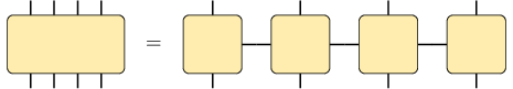
In graphical notation, mpo looks like this

It’s basic properties are:

[len(mpo), mpo.ndims, mpo.ranks]

[4, (2, 2, 2, 2), (3, 3, 3)]

Each site has two physical legs, one with dimension 3 and one with dimension 2. This corresponds to a non-square full array.

mpo.shape

((3, 2), (3, 2), (3, 2), (3, 2))

Now convert the mpo to a full array:

mpo_arr = mpo.to_array()
mpo_arr.shape

(3, 2, 3, 2, 3, 2, 3, 2)

We refer to this arangement of axes as local form, since indices which correspond to the same site are neighboring. This is a natural form for the MPO representation. However, for some operations it is necessary to have row and column indices grouped together – we refer to this as global form:

from mpnum.utils.array_transforms import local_to_global

mpo_arr = mpo.to_array()
mpo_arr = local_to_global(mpo_arr, sites=len(mpo))
mpo_arr.shape

(3, 3, 3, 3, 2, 2, 2, 2)

This gives the expected result. Note that it is crucial to specify the correct number of sites, otherwise we do not get what we want:

mpo_arr = mpo.to_array()
mpo_arr = local_to_global(mpo_arr, sites=2)
mpo_arr.shape

(3, 3, 2, 2, 3, 3, 2, 2)

As an alternative, there is the following shorthand:

mpo_arr = mpo.to_array_global()
mpo_arr.shape

(3, 3, 3, 3, 2, 2, 2, 2)

An array in global form can be converted into matrix-product form with the following API:

mpo2 = mp.MPArray.from_array_global(mpo_arr, ndims=2)
mp.normdist(mpo, mpo2)

1.0881840590136613e-15

MPO-MPS product and arbitrary MPA-MPA products

We can now compute the matrix-vector product of mpa from above (which is an MPS) and mpo.

mpa.shape

((2,), (2,), (2,), (2,))

mpo.shape

((3, 2), (3, 2), (3, 2), (3, 2))

prod = mp.dot(mpo, mpa, axes=(-1, 0))
prod.shape

((3,), (3,), (3,), (3,))

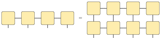
The result is a new MPS, with local dimension changed by mpo and looks like this:

The axes argument is optional and defaults to axes=(-1, 0) – i.e. contracting, at each site, the last pyhsical index of the first factor with the first physical index of the second factor. More specifically, the axes argument specifies which physical legs should be contracted: axes[0] specifies the physical in the first argument, and axes[1] specifies the physical leg in the second argument. This means that the same product can be achieved with

prod2 = mp.dot(mpa, mpo, axes=(0, 1))
mp.normdist(prod, prod2)

1.7794893594008944e-16

Note that in any case, the ranks of the output of mp.dot are the products of the original ranks:

mpo.ranks, mpa.ranks, prod.ranks

((3, 3, 3), (2, 3, 2), (6, 9, 6))

Now we compute the same product using the full arrays arr and mpo_arr:

arr_vec = arr.ravel()
mpo_arr = mpo.to_array_global()
mpo_arr_matrix = mpo_arr.reshape((81, 16))
prod3_vec = np.dot(mpo_arr_matrix, arr_vec)
prod3_vec.shape

(81,)

As you can see, we need to reshape the result prod3_vec before we can convert it back to an MPA:

prod3_arr = prod3_vec.reshape((3, 3, 3, 3))
prod3 = mp.MPArray.from_array(prod3_arr, ndims=1)
prod3.shape

((3,), (3,), (3,), (3,))

Now we can compare the two results:

mp.normdist(prod, prod3)

2.0433926816958574e-16

We can also compare by converting prod to a full array:

prod_arr = prod.to_array()
la.norm((prod3_arr - prod_arr).reshape(81))

1.0434960119970279e-16

Converting full operators to MPOs

While MPO algorithms avoid using full operators in general, we will need to convert a term acting on only two sites to an MPO in order to continue with MPO operations; i.e. we will need to convert a full array to an MPO.

First, we define a full operator:

CZ = np.array([[ 1.,  0.,  0.,  0.],
               [ 0.,  1.,  0.,  0.],
               [ 0.,  0.,  1.,  0.],
               [ 0.,  0.,  0., -1.]])

This operator is the so-called controlled Z gate: Apply Z on the second qubit if the first qubit is in state e2.

To convert it to an MPO, we have to reshape:

CZ_arr = CZ.reshape((2, 2, 2, 2))

Now we can create an MPO, being careful to specify the correct number of legs per site:

CZ_mpo = mp.MPArray.from_array_global(CZ_arr, ndims=2)

To test it, we apply the operator to the state which has both qubits in state e2:

vec = np.kron([0, 1], [0, 1])
vec

array([0, 0, 0, 1])

Reshape and convert to an MPS:

vec_arr = vec.reshape([2, 2])
mps = mp.MPArray.from_array(vec_arr, ndims=1)

Now we can compute the matrix-vector product:

out = mp.dot(CZ_mpo, mps)
out.to_array().ravel()

array([ 0.,  0.,  0., -1.])

The output is as expected: We have acquired a minus sign.

We have to be careful to use from_array_global and not from_array for CZ_mpo, because the CZ_arr is in global form. Here, all physical legs have the same dimension, so we can use from_array without error:

CZ_mpo2 = mp.MPArray.from_array(CZ_arr, ndims=2)

However, the result is not what we want:

out2 = mp.dot(CZ_mpo2, mps)
out2.to_array().ravel()

array([ 1.,  0.,  0., -1.])

The reason is easy to see: We have applied the following matrix to our state:

CZ_mpo2.to_array_global().reshape(4, 4)

array([[ 1.,  0.,  0.,  1.],
       [ 0.,  0.,  0.,  0.],
       [ 0.,  0.,  0.,  0.],
       [ 1.,  0.,  0., -1.]])

Keep in mind that we have to use to_array_global before the reshape. Using to_array would not provide us the matrix which we have applied to the state with mp.dot. Instead, it will exactly return the input:

CZ_mpo2.to_array().reshape(4, 4)

array([[ 1.,  0.,  0.,  0.],
       [ 0.,  1.,  0.,  0.],
       [ 0.,  0.,  1.,  0.],
       [ 0.,  0.,  0., -1.]])

Again, from_array_global is just the shorthand for the following:

from mpnum.utils.array_transforms import global_to_local

CZ_mpo3 = mp.MPArray.from_array(global_to_local(CZ_arr, sites=2), ndims=2)

mp.normdist(CZ_mpo, CZ_mpo3)

1.5700924586837752e-16

As you can see, in the explicit version you must submit both the correct number of sites and the correct number of physical legs per site. Therefore, the function MPArray.from_array_global simplifies the conversion.

Creating MPAs from Kronecker products

It is a frequent task to create an MPS which represents the product state of \(\vert 0 \rangle\) on each qubit. If the chain is very long, we cannot create the full array with np.kron and use MPArray.from_array afterwards because the array would be too large.

In the following, we describe how to efficiently construct an MPA representation of a Kronecker product of vectors. The same methods can be used to efficiently construct MPA representations of Kronecker products of operators or tensors with three or more indices.

First, we need the state on a single site:

e1 = np.array([1, 0])
e1

array([1, 0])

Then we can use from_kron to directly create an MPS representation of the Kronecker product:

mps = mp.MPArray.from_kron([e1, e1, e1])
mps.to_array().ravel()

array([1, 0, 0, 0, 0, 0, 0, 0])

This works well for large numbers of sites because the needed memory scales linearly with the number of sites:

mps = mp.MPArray.from_kron([e1] * 2000)
len(mps)

2000

An even more pythonic solution is the use of iterators in this example:

from itertools import repeat

mps = mp.MPArray.from_kron(repeat(e1, 2000))
len(mps)

2000

Do not call .to_array() on this state!

The bond dimension of the state is 1, because it is a product state:

np.array(mps.ranks)  # Convert to an array for nicer display

array([1, 1, 1, ..., 1, 1, 1])

We can also create a single-site MPS:

mps1 = mp.MPArray.from_array(e1, ndims=1)
len(mps1)

1

After that, we can use mp.chain to create Kronecker products of the MPS directly:

mps = mp.chain([mps1, mps1, mps1])
len(mps)

3

It returns the same result as before:

mps.to_array().ravel()

array([1, 0, 0, 0, 0, 0, 0, 0])

We can also use mp.chain on the three-site MPS:

mps = mp.chain([mps] * 100)
len(mps)

300

Note that mp.chain interprets the factors in the tensor product as distinct sites. Hence, the factors do not need to be of the same length or even have the same number of indices. In contrast, there is also mp.localouter, which computes the tensor product of MPArrays with the same number of sites:

mps = mp.chain([mps1] * 4)
len(mps), mps.shape,

(4, ((2,), (2,), (2,), (2,)))

rho = mp.localouter(mps.conj(), mps)
len(rho), rho.shape

(4, ((2, 2), (2, 2), (2, 2), (2, 2)))

Compression

A typical matrix product based numerical algorithm performs many additions or multiplications of MPAs. As mentioned above, both operations increase the rank. If we let the bond dimension grow, the amount of memory we need grows with the number of operations we perform. To avoid this problem, we have to find an MPA with a smaller rank which is a good approximation to the original MPA.

We start by creating an MPO representation of the identity matrix on 6 sites with local dimension 3:

op = mp.eye(sites=6, ldim=3)

op.shape

((3, 3), (3, 3), (3, 3), (3, 3), (3, 3), (3, 3))

As it is a tensor product operator, it has rank 1:

op.ranks

(1, 1, 1, 1, 1)

However, addition increases the rank:

op2 = op + op + op
op2.ranks

(3, 3, 3, 3, 3)

Matrix multiplication multiplies the individual ranks:

op3 = mp.dot(op2, op2)
op3.ranks

(9, 9, 9, 9, 9)

(NB: compress or compression below can call canonicalize on the MPA, which in turn could already reduce the rank to 1 in case the rank can be compressed without error. Keep that in mind.)

Keep in mind that the operator represented by op3 is still the identity operator, i.e. a tensor product operator. This means that we expect to find a good approximation with low rank easily. Finding such an approximation is called compression and is achieved as follows:

op3 /= mp.norm(op3.copy())  # normalize to make overlap meaningful
copy = op3.copy()
overlap = copy.compress(method='svd', rank=1)
copy.ranks

(1, 1, 1, 1, 1)

Calling compress on an MPA replaces the MPA in place with a version with smaller bond dimension. Overlap gives the absolute value of the (Hilbert-Schmidt) inner product between the original state and the output:

overlap

0.99999999999999911

Instead of in-place compression, we can also obtain a compressed copy:

compr, overlap = op3.compression(method='svd', rank=2)
overlap, compr.ranks, op3.ranks

(0.99999999999999911, (2, 2, 2, 2, 2), (9, 9, 9, 9, 9))

SVD compression can also be told to meet a certain truncation error (see the documentation of mp.MPArray.compress for details).

compr, overlap = op3.compression(method='svd', relerr=1e-6)
overlap, compr.ranks, op3.ranks

(0.99999999999999911, (1, 1, 1, 1, 1), (9, 9, 9, 9, 9))

We can also use variational compression instead of SVD compression:

compr, overlap = op3.compression(method='var', rank=2, num_sweeps=10, var_sites=2)
# Convert overlap from numpy array with shape () to float for nicer display:
overlap = overlap.flat[0]
complex(overlap), compr.ranks, op3.ranks

((1+0j), (2, 2, 2, 2, 2), (9, 9, 9, 9, 9))

As a reminder, it is always advisable to check whether the overlap between the input state and the compression is large enough. In an involved algorithm, it can be useful to store the compression error at each invocation of compression.

MPO sum of local terms

A frequent task is to compute the MPO representation of a local Hamiltonian, i.e. of an operator of the form

\[ \begin{align}\begin{aligned}H = \sum_{i=1}^{n-1} h_{i, i+1}\\where :math:`h_{i, i+1}` acts only on sites :math:`i` and\end{aligned}\end{align} \]

\(i + 1\). This means that \(h_{i, i+1} = \mathbb 1_{i - 1} \otimes h'_{i, i+1} \otimes \mathbb 1_{n - w + 1}\) where \(\mathbb 1_k\) is the identity matrix on \(k\) sites and \(w = 2\) is the width of \(h'_{i, i+1}\).

We show how to obtain an MPO representation of such a Hamiltonian. First of all, we need to define the local terms. For simplicity, we choose \(h'_{i, i+1} = \sigma_Z \otimes \sigma_Z\) independently of \(i\).

zeros = np.zeros((2, 2))
zeros

array([[ 0.,  0.],
       [ 0.,  0.]])

idm = np.eye(2)
idm

array([[ 1.,  0.],
       [ 0.,  1.]])

# Create a float array instead of an int array to avoid problems later
Z = np.diag([1., -1])
Z

array([[ 1.,  0.],
       [ 0., -1.]])

h = np.kron(Z, Z)
h

array([[ 1.,  0.,  0.,  0.],
       [ 0., -1.,  0., -0.],
       [ 0.,  0., -1., -0.],
       [ 0., -0., -0.,  1.]])

First, we have to convert the local term h to an MPO:

h_arr = h.reshape((2, 2, 2, 2))
h_mpo = mp.MPArray.from_array_global(h_arr, ndims=2)
h_mpo.ranks

(4,)

h_mpo has rank 4 even though h is a tensor product. This is far from optimal. We improve things as follows: (We could also compress h_mpo.)

h_mpo = mp.MPArray.from_kron([Z, Z])
h_mpo.ranks

(1,)

The most simple way is to implement the formula from above with MPOs: First we compute the \(h_{i, i+1}\) from the \(h'_{i, i+1}\):

width = 2
sites = 6
local_terms = []

for startpos in range(sites - width + 1):
    left = [mp.MPArray.from_kron([idm] * startpos)] if startpos > 0 else []
    right = [mp.MPArray.from_kron([idm] * (sites - width - startpos))] \
        if sites - width - startpos > 0 else []
    h_at_startpos = mp.chain(left + [h_mpo] + right)
    local_terms.append(h_at_startpos)

local_terms

[<mpnum.mparray.MPArray at 0x7f6563b08588>,
 <mpnum.mparray.MPArray at 0x7f6563b084e0>,
 <mpnum.mparray.MPArray at 0x7f6563b086a0>,
 <mpnum.mparray.MPArray at 0x7f6563b08710>,
 <mpnum.mparray.MPArray at 0x7f6563b08630>]

Next, we compute the sum of all the local terms and check the bond dimension of the result:

H = local_terms[0]

for local_term in local_terms[1:]:
    H += local_term

H.ranks

(5, 5, 5, 5, 5)

The ranks are explained by the ranks of the local terms:

[local_term.ranks for local_term in local_terms]

[(1, 1, 1, 1, 1),
 (1, 1, 1, 1, 1),
 (1, 1, 1, 1, 1),
 (1, 1, 1, 1, 1),
 (1, 1, 1, 1, 1)]

We just have to add the ranks at each position.

mpnum provides a function which constructs H from h_mpo, with an output MPO with smaller rank by taking into account the trivial action on some sites:

H2 = mp.local_sum([h_mpo] * (sites - width + 1))
H2.ranks

(2, 3, 3, 3, 2)

Without additional arguments, mp.local_sum() just adds the local terms with the first term starting on site 0, the second on site 1 and so on. In addition, the length of the chain is chosen such that the last site of the chain coincides with the last site of the last local term. Other constructions can be obtained by prodividing additional arguments.

We can check that the two Hamiltonians are equal:

mp.normdist(H, H2)

6.4354640488548389e-15

Of course, this means that we could just compress H:

H_comp, overlap = H.compression(method='svd', rank=3)
overlap / mp.norm(H)**2

0.99999999999999889

H_comp.ranks

(3, 3, 3, 3, 3)

We can also check the minimal bond dimension which can be achieved with SVD compression with small error:

H_comp, overlap = H.compression(method='svd', relerr=1e-6)
overlap / mp.norm(H)**2

0.99999999999999933

H_comp.ranks

(2, 3, 3, 3, 2)

MPS, MPOs and PMPS

We can represent vectors (e.g. pure quantum states) as MPS, we can represent arbitrary matrices as MPO and we can represent positive semidefinite matrices as purifying matrix product states (PMPS). For mixed quantum states, we can thus choose between the MPO and PMPS representations.

As mentioned in the introduction, MPS and MPOs are handled as MPAs with one and two physical legs per site. In addition, PMPS are handled as MPAs with two physical legs per site, where the first leg is the “system” site and the second leg is the corresponding “ancilla” site.

From MPS and PMPS representations, we can easily obtain MPO representations. mpnum provides routines for this:

mps = mp.random_mpa(sites=5, ldim=2, rank=3, normalized=True)
mps_mpo = mp.mps_to_mpo(mps)
mps_mpo.ranks

(4, 9, 9, 4)

As expected, the rank of mps_mpo is the square of the rank of mps.

Now we create a PMPS with system site dimension 2 and ancilla site dimension 3:

pmps = mp.random_mpa(sites=5, ldim=(2, 3), rank=3, normalized=True)
pmps.shape

((2, 3), (2, 3), (2, 3), (2, 3), (2, 3))

pmps_mpo = mp.pmps_to_mpo(pmps)
pmps_mpo.ranks

(9, 9, 9, 9)

Again, the rank is squared, as expected. We can verify that the first physical leg of each site of pmps is indeed the system site by checking the shape of pmps_mpo:

pmps_mpo.shape

((2, 2), (2, 2), (2, 2), (2, 2), (2, 2))

Local reduced states

For state tomography applications, we frequently need the local reduced states of an MPS, MPO or PMPS. We provide the following functions for this task:

• mp.reductions_mps_as_pmps(): Input: MPS, output: local reductions as PMPS
• mp.reductions_mps_as_mpo(): Input: MPS, output: local reductions as MPO
• mp.reductions_pmps(): Input: PMPS, output: Local reductions as PMPS
• mp.reductions_mpo(): Input: MPO, output: Local reductions as MPO

The arguments of all functions are similar, e.g.:

width = 3
startsites = range(len(pmps) - width + 1)
for startsite, red in zip(startsites, mp.reductions_pmps(pmps, width, startsites)):
    print('Reduction starting on site', startsite)
    print('bdims:', red.ranks)
    red_mpo = mp.pmps_to_mpo(red)
    print('trace:', mp.trace(red_mpo))
    print()

Reduction starting on site 0
bdims: (3, 3)
trace: 1.0

Reduction starting on site 1
bdims: (3, 3)
trace: 1.0

Reduction starting on site 2
bdims: (3, 3)
trace: 1.0

Because pmps was a normalized state, the trace of the reduced states is close to 1.

You can omit the startsites argument: The default behaviour is the first reductions starting on site 0, the second on site 1, and so on (which is just what we have requested). The functions for reduced states can also compute different constructions by providing different arguments not described here.